ALLSHIFT/Shift Matlab Drive/Shift Matlab Drive/Simulations/Exisiting EST Model/est-model-main/EST-model-main/README.md

EST-model

This project contains the Simulink model for the Energy Storage and Transport (EST) project. This Simulink model contains a simplified version of a real-life energy storage and transport system, which describes the flow of energy in such a system. Supporting MATLAB files are provided which can be used to predefine parameters and to post-process data into figures.

Getting started

To install the simulink model, just clone or download the entire repository (under <> Code) and open EST.slx. If you download the zip file for the repository, make sure to properly unzip it, as otherwise errors occur.

Version requirements

The simulink model EST.slx requires Matlab R2022b or newer, with the Simulink toolbox installed. Older, untested, versions are available in the versions directory. In order to run an older version, copy the Simulink file corresponding to your version into the main directory and make sure to restart both MATLAB and Simulink before running it.

Overview of files and directory structure

• EST.slx: Main file, containing the runnable Simulink model of the EST system.
• preprocessing.m: Matlab script to define the model parameters and to read the supply and demand data files. Automatically executed by the Simulink model before running.
• postprocessing.m: Matlab script to plot the model results. Automatically executed by the Simulink model after running.
• data directory: Directory from which the supply and demand data is to be read. By default, the directory contains example files for a storage system in a household with solar panels (see Running the model), and the files for a charge/discharge cycle (see Charge/discharge cycle).

Running the model

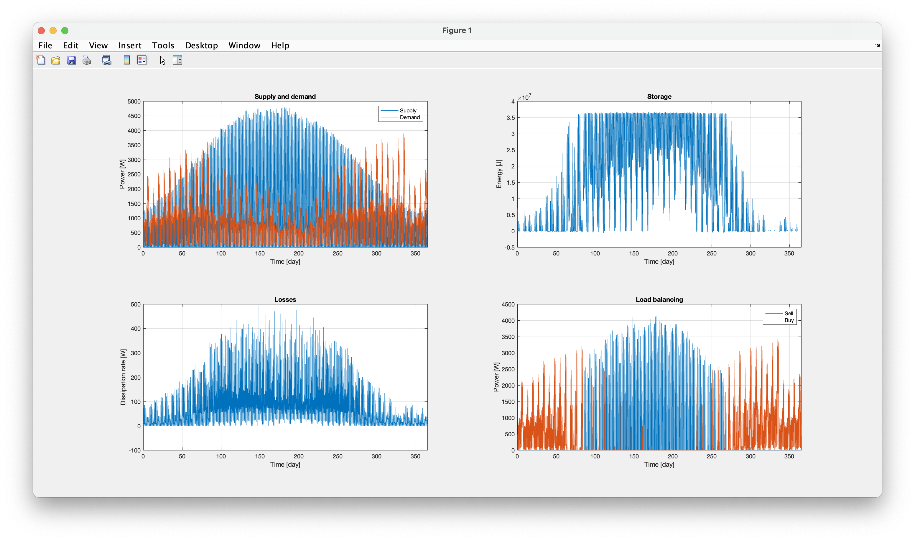
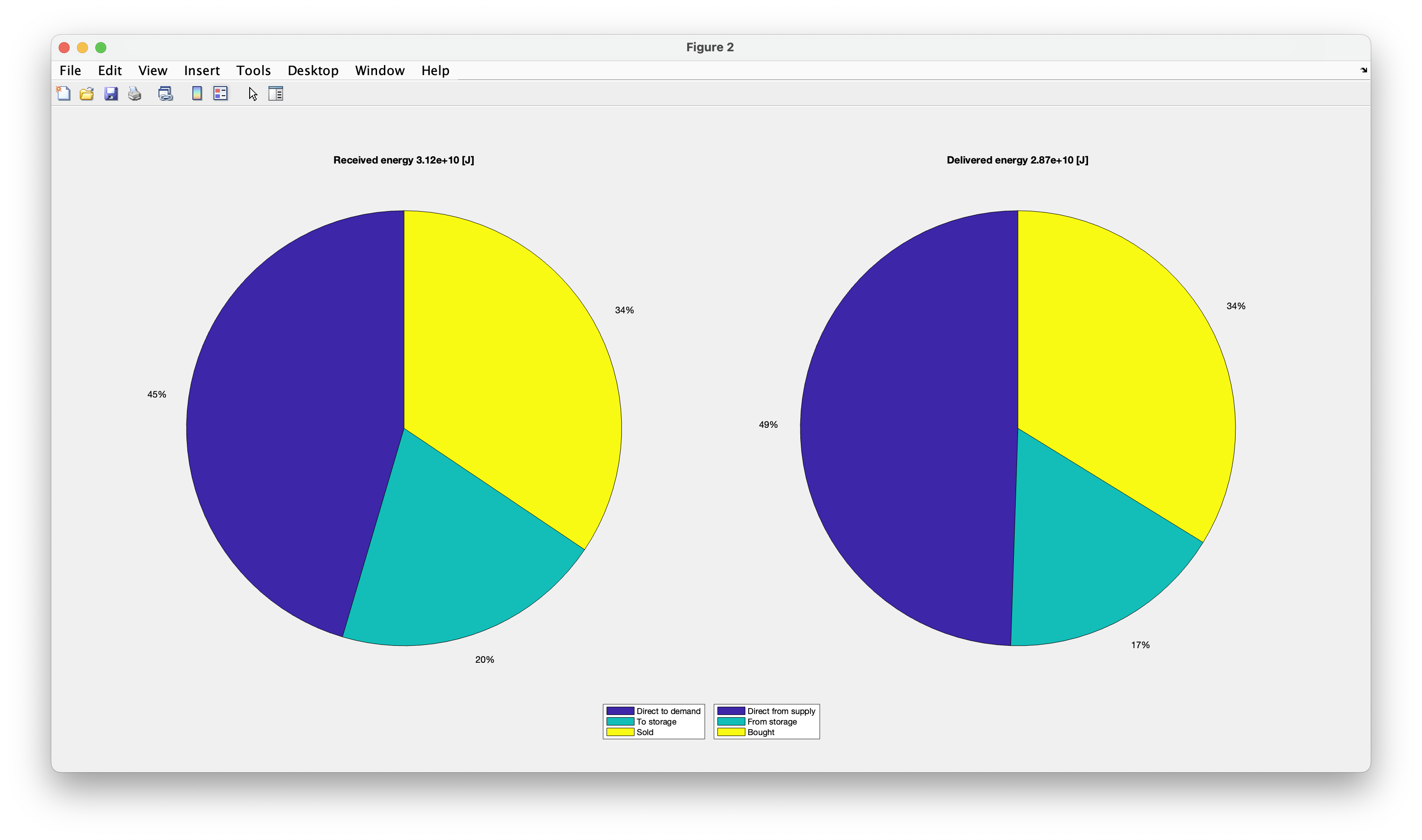
To run the model, open EST.slx and click the run button: 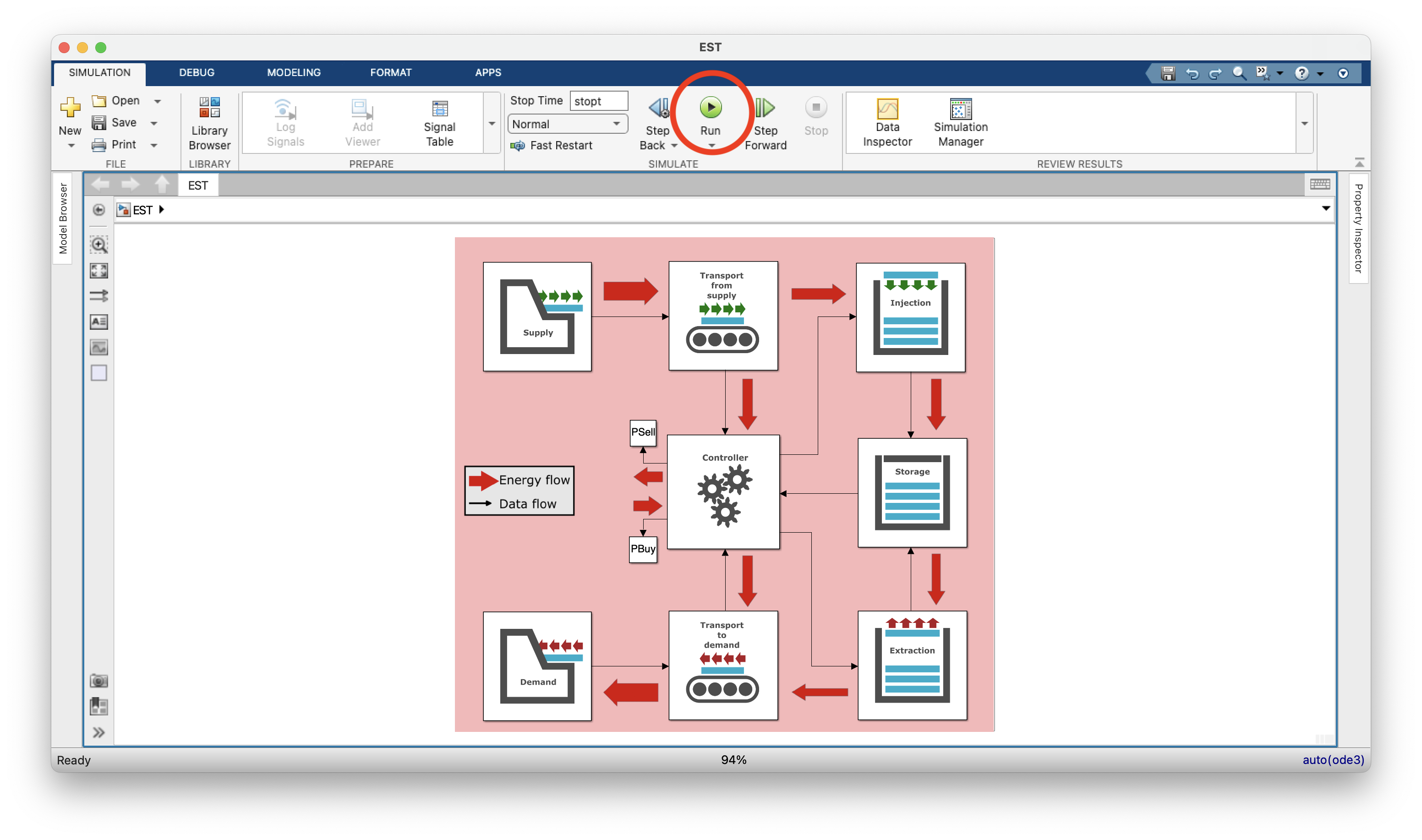After running is complete, the following output is displayed:

Caution

When the code gives an error, carefully check the following:

• Did you install the complete repository? Only downloading EST.slx does not work.
• If you downloaded the zip file, did you unpack it?
• Is the Matlab current working directory set to the right folder, that is, the folder in which EST.slx is placed.

The results displayed above correspond to the default model settings, as configured in the preprocessing.m Matlab script:

% Pre-processing script for the EST Simulink model. This script is invoked
% before the Simulink model starts running (initFcn callback function).

%% Load the supply and demand data

timeUnit   = 's';

supplyFile = "SolarExample_supply.csv";
supplyUnit = "kW";

% load the supply data
Supply = loadSupplyData(supplyFile, timeUnit, supplyUnit);

demandFile = "SolarExample_demand.csv";
demandUnit = "kW";

% load the demand data
Demand = loadDemandData(demandFile, timeUnit, demandUnit);

%% Simulation settings

deltat = 5*unit("min");
stopt  = min([Supply.Timeinfo.End, Demand.Timeinfo.End]);

%% System parameters

% transport from supply
aSupplyTransport = 0.01; % Dissipation coefficient

% injection system
aInjection = 0.1; % Dissipation coefficient

% storage system
EStorageMax     = 10.*unit("kWh"); % Maximum energy
EStorageMin     = 0.0*unit("J");   % Minimum energy
EStorageInitial = 2.0*unit("kWh"); % Initial energy
bStorage        = 1e-6/unit("s");  % Storage dissipation coefficient

% extraction system
aExtraction = 0.1; % Dissipation coefficient

% transport to demand
aDemandTransport = 0.01; % Dissipation coefficient

Theory and implementation

The EST system transports energy from the Supply to the Demand, both represented by a block in the Simulink model, possibly storing the energy in between. The EST model consists of five components (blocks), in the order of the energy flow:

1. Transport from supply: transports the energy from the supply site to the storage site.
2. Injection: inserts energy into the storage container.
3. Storage: container in which the energy is stored.
4. Extraction: extracts energy from the storage container.
5. Transport to demand: transports the energy from the storage site to the demand site.

The flow of energy between these components is managed by a controller, which ensures that the electrical power balance is satisfied through load balancing (buying or selling of energy).

Each subsystem in the model can be described by

\dot{E}=P_{\rm in}-P_{\rm out}-D

where \dot{E} is the change of total energy in the subsystem, P_{\rm in} the incoming power, P_{\rm out} the outgoing power and D the rate of dissipation in the subsystem.

For the Transport from supply, Injection, Extractionand Transport to demand components, the EST model assumes \dot{E}=0 and

D= a P_{\rm in}

where a [-] is the subsystem dissipation coefficients. It then follows that

P_{\rm out} = P_{\rm in} - D = (1-a) P_{\rm in}

These relations are implemented in Simulink through Matlab function blocks, for example for the Injection component:

function [PfromInjection, DInjection] = injection(PtoInjection, aInjection)
    DInjection = aInjection * PtoInjection;
    PfromInjection = PtoInjection - DInjection;

Note that P_{\rm in} and P_{\rm out} are here represented by PtoInjection and PfromInjection, respectively. The Transport from supply component follows the same implementation:

function [PfromSupplyTransport, DSupplyTransport] = supplyTransport(PtoSupplyTransport, aSupplyTransport)
    DSupplyTransport = aSupplyTransport * PtoSupplyTransport;
    PfromSupplyTransport = PtoSupplyTransport - DSupplyTransport;

When P_{\rm out} serves as the input of the system, for example for the Extraction component, the dissipation and power functions must be rewritten to

D = \frac{a}{1-a} P_{\rm out}

and

P_{\rm in} = P_{\rm out} + D = \frac{1}{1-a} P_{\rm out}

The implementation then follows as:

function [PtoExtraction, DExtraction] = extraction(PfromExtraction, aExtraction)
    DExtraction = aExtraction / (1-aExtraction) * PfromExtraction;
    PtoExtraction = PfromExtraction + DExtraction;

Similarly, for the Transport to demand component, the implementation reads:

function [PtoDemandTransport, DDemandTransport] = demandTransport(PfromDemandTransport, aDemandTransport)
    DDemandTransport = aDemandTransport / (1-aDemandTransport) * PfromDemandTransport;
    PtoDemandTransport = PfromDemandTransport + DDemandTransport;

For the Storage component, the dissipation model

D= b (E - E_{\rm min})

is assumed, where E_{\rm min} is the minimum energy capacity of the system (by default set to 0) and b [1/s] is the storage dissipation coefficient. This model essential states that the dissipation is proportional to the amount of energy stored.

Substitution of this dissipation model in the power balance results in the differential equation (DE)

\dot{E} + b E =P_{\rm in}-P_{\rm out}+b E_{\rm min}

In the Simulink model, this differential equation is integrated explicitly, meaning that \dot{E} is computed based on the energy E in the previous time step:

function [DStorage, EdotStorage]= Storage(PtoStorage, PfromStorage, bStorage, aStorage , EStorageMin, EStorage)
    DStorage = bStorage * (EStorage-EStorageMin);
    EdotStorage = PtoStorage - PfromStorage - DStorage;

Charge/discharge cycle

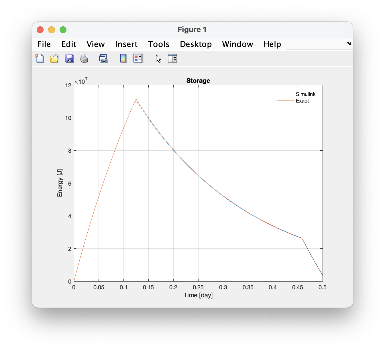
To illustrate the theory behind the model, we consider a single charge/discharge cycle. In this cycle, the energy system is charged for T_{\rm charge}=3 [h] with a power of P_{\rm charge}=15 [kW], after which the energy is stored for T_{\rm store}=8 [h], until the system is discharged for T_{\rm discharge}=1 [h] with a power of P_{\rm discharge}=5 [kW]. The corresponding supply and demand signals are stored in the CycleExample_supply.csv and CycleExample_demand.csv files. To read these files, the preprocessing.m file is configured as:

% Pre-processing script for the EST Simulink model. This script is invoked
% before the Simulink model starts running (initFcn callback function).

%% Load the supply and demand data

timeUnit   = 's';

supplyFile = "CycleExample_supply.csv";
supplyUnit = "kW";

% load the supply data
Supply = loadSupplyData(supplyFile, timeUnit, supplyUnit);

demandFile = "CycleExample_demand.csv";
demandUnit = "kW";

% load the demand data
Demand = loadDemandData(demandFile, timeUnit, demandUnit);

The time step size, deltat, used in the simulation is also specified in preprocessing.m and the final simulation time, stopt, is determined from the loaded time series:

%% Simulation settings

deltat = 5*unit("min");
stopt  = min([Supply.Timeinfo.End, Demand.Timeinfo.End]);

Finally, the dissipation coefficients are given by:

%% System parameters

% transport from supply
aSupplyTransport = 0.01; % Dissipation coefficient

% injection system
aInjection = 0.1; % Dissipation coefficient

% storage system
EStorageMax     = 40*unit("kWh"); % Maximum energy
EStorageMin     = 0.0*unit("J");  % Minimum energy
EStorageInitial = 0.0*unit("J");  % Initial energy
bStorage        = 5e-5/unit('s'); % Storage dissipation coefficient

% extraction system
aExtraction = 0.1; % Dissipation coefficient

% transport to demand
aDemandTransport = 0.01; % Dissipation coefficient

For this particular scenario, an exact solution to the model exists, which can be used to verify the Simulink implementation. During charging, the power balance differential equation for the storage container reads

\dot{E} + b E = c P_{\rm supply}

where c = (1-a_{\rm supplyTransport}) (1-a_{\rm Injection}). With the initial condition E(0)=0, the solution is given by

E = (1 - e^{-bt}) \frac{c}{b} P_{\rm supply} \qquad 0 \leq t < T_{\rm charge}

During storage, the power balance reads

\dot{E} + b E = 0

with the initial condition E(T_{\rm charge}) = (1 - e^{-bT_{\rm charge}}) \frac{c}{b} P_{\rm supply} := E_{\rm charge}. The solution during storage is given by

E = E_{\rm charge} e^{-b(t - T_{\rm charge})} \qquad T_{\rm charge} \leq t \leq \tau

where \tau = T_{\rm charge} + T_{\rm store}. Finally, during discharging, the differential equation reads

\dot{E} + b E = -d P_{\rm demand}

where d = (1-a_{\rm Extraction})^{-1}(1-a_{\rm demandTransport})^{-1}. With the initial condition E(\tau)=E_{\rm charge} e^{-b T_{\rm store}} := E_{\rm store}, the solution is given by

E = (e^{-b(t-\tau)} -1) \frac{d}{b} P_{\rm demand} + E_{\rm store} e^{-b(t-\tau)} \qquad \tau \leq t \leq \tau + T_{\rm discharge}

Comparison of this exact solution with the Simulink model conveys that the model solves the model equations as intended: